Sequins Metagenomics Core Control Set Tutorial: Reference-based quantification of known targets
This is an example workflow for processing short-read metagenomics sequencing data from samples which have had the Sequins Metagenomics Core Control Set spiked in. It highlights the places where Sequins-specific steps must be taken, and it is not intended as an example of a production workflow. You should adapt each step to your own needs.
Obtain the tutorial resources
The necessary files to run this tutorial, including the Sequins resource bundle and example sequencing data, can be obtained by completing the request access form.
Sequins resource bundle
The provided user bundle contains the following reference files:
-
metasequin_sequences.fa: A standard multi-FASTA file containing individual synthetic metagenomic sequences (Sequins), each represented as a separate FASTA entry. -
metasequin_decoy.fa: A concatenated version of the same sequences frommetasequin_sequences.fabut merged into a single pseudochromosome-style FASTA entry, with individual sequences separated by a stretch of N bases. This format facilitates compatibility with alignment tools that require a linear reference and is designed to be used in conjunction with the accompanying BED file. -
metasequin_regions.bed: Provides the precise coordinates demarcating the boundaries of each individual sequin withinmetasequin_decoy.fa. -
metasequin_abundances.csv: The abundance column represents the relative molar proportion of each Sequins control in the mixture — i.e. how much of each Sequins control was included in relation to the others. Once you know the total amount of Sequins spiked in (e.g. 1 ng), you can use these values to calculate the expected mass of each individual Sequins control. In other words, the abundance value does not represent an absolute unit like ng or copies/µL, but rather a proportional value to guide normalisation or expected abundance calculations. The length field is in base pairs (bp).
Tutorial example data
Sequins provides example data derived from short-read sequencing of a dog’s microbiome, subset to reduce file size for testing with the workflow. The files for running the tutorial include:
-
microbial_genomes.fa: A standard multi-FASTA file containing the reference genomes of the microbial target species. -
meta_tutorial_data_v1.1_R1.fastq.gz,meta_tutorial_data_v1.1_R2.fastq.gz: Raw FASTQ files for the example sample. -
metasequin_abundances_example.csv: A file with pre-computed ng/µL and copies/µL values for each Sequins control in the sample. -
functions.py: Python helper functions for normalising quantified read counts, plotting Sequins ladders, and calculating limit of detection/quantification.
Intermediary files from each analysis stage are included in the intermediatory_files/ directory to allow continuation of the tutorial if any issues arise (e.g. tool installation or runtime errors). These include:
- Combined microbial + Sequins reference genome and all associated index files.
- FASTQ files after quality processing, plus associated reports.
- The aligned BAM file and its index.
- Quantified abundances generated with bedtools multicov.
- Outputs from the downstream Python analysis of quantified Sequins.
Prepare your environment
Option 1: Self-serve comprehensive
Sequins provides a Docker container that has all dependencies pre-installed, this is the recommended way to run this tutorial. You can download the latest version of the image with:
docker pull ghcr.io/sequinsbio/meta_tutorial:1.1.0
NOTE: The Docker container only supports x86_64 architectures. If you’re running this tutorial on an ARM64 architecture (e.g., Apple Silicon), you should set the
DOCKER_DEFAULT_PLATFORMenvironment variable tolinux/amd64before running any Docker commands. This ensures that the container runs in an x86_64 emulation mode, which is necessary for compatibility with the tools included in the container.export DOCKER_DEFAULT_PLATFORM=linux/amd64Alternatively, you can add the option
--platform linux/amd64to every Docker command.
Option 2: Independent tools
Alternatively, if you are unable to run Docker or would prefer to run the tools natively, you can install each dependency locally.
In this example workflow we use a number of popular bioinformatics tools that need to be installed. However, users should feel free to use alternative software tools and/or versions to suit their needs.
Running the workflow
The following steps will walk you through a basic workflow for quantifying abundance from shotgun metagenomic sequencing in detail, so you can follow along either running inside the 1) Docker container or 2) on your local machine. You can start the Docker container with:
docker run -it --rm -v "$PWD":"$PWD" -w "$PWD" -u "$(id -u)":"$(id -g)" \
   ghcr.io/sequinsbio/meta_tutorial:1.1.0
1. Build a Sequins augmented reference genome
This step only needs to be performed once, and the resulting FASTA file can be used for all subsequent analyses which target the same microbial species.
To prepare a reference for alignment-based quantification for use with
an aligner such as BWA-mem, you can simply concatenate metasequin_sequences.fa
to the reference genomes for the microbial species of interest and prepare the relevant index files:
cat meta_tutorial_data_v1.1/microbial_reference.fa \
    metagenomics_core_control_set_v2/metasequin_sequences.fa \
    > microbial_with_sequins.fa
samtools faidx microbial_with_sequins.fa
samtools dict microbial_with_sequins.fa > microbial_with_sequins.dict
bwa index microbial_with_sequins.fa
faidx --transform bed microbial_with_sequins.fa > microbial_with_sequins.bed
2. Perform quality control of raw sequencing data
Whether quality control and pre-processing is necessary and to what extent is dataset-specific and as such, tools and parameters should be selected accordingly. Below is an example of adaptor trimming and quality filtering of raw sequencing data with fastp:
fastp --in1 meta_tutorial_data_v1.1/meta_tutorial_data_v1.1_R1.fastq.gz \
    --in2 meta_tutorial_data_v1.1/meta_tutorial_data_v1.1_R2.fastq.gz \
    --out1 meta_tutorial_data_v1.1_R1.qc.fastq.gz \
    --out2 meta_tutorial_data_v1.1_R2.qc.fastq.gz \
    -q 20 -l 36 \
    --correction \
    --cut_tail \
    --trim_poly_x \
    --trim_poly_g \
    --json meta_tutorial_data_v1.1.fastp.json \
    --html meta_tutorial_data_v1.1.fastp.html
You may optionally consider removal of host DNA and/or PhiX if relevant for the sample, however this step has been performed already for the example data provided with this tutorial.
3. Abundance quantification
To perform an alignment with BWA:
bwa mem -M -t 8 -R "@RG\\tID:A\\tSM:A\\tLB:libA\\tPU:puA\\tPL:ILLUMINA" \
    microbial_with_sequins.fa \
    meta_tutorial_data_v1.1_R1.qc.fastq.gz \
    meta_tutorial_data_v1.1_R2.qc.fastq.gz |
    samtools fixmate -u -m - - |
    samtools sort -u - |
    samtools markdup -u - - |
    samtools view -b > meta_tutorial_data_v1.1.bam
samtools index meta_tutorial_data_v1.1.bam
You can then calculate abundance for each Sequins and microbial species
in the reference with your preferred tool. Here we demonstrate
quantification with the bedtools multicov command:
bedtools multicov \
    -bams meta_tutorial_data_v1.1.bam \
    -bed microbial_with_sequins.bed \
    -D \
    -p \
    -q 1 \
    > meta_tutorial_data_v1.1.coverage.txt
4. Downstream analysis with Sequins
4.1 Calculating expected input of Sequins
As the abundance value provided (e.g. 32,768 for SQN000000141) in the
metasequin_abundances.csv file reflects the relative abundance within
the mix of 65 Sequins, this value can be used to calculate the expected
input for the linear regression.
In the example data provided with this tutorial, Sequins was spiked into a 10 µL sample containing 37.7 ng of DNA at 1%, resulting in a total of 0.377 ng input, or 0.03427 ng/µL in the final 11 µL of spiked-in sample. With these values we can work out the ng/µL (or total ng if preferred) of each Sequins control, , using the following formula:
For example, for Sequins control SQN000000141 in this dataset, this would be:
This approach ensures that the contribution of each Sequins control to the total mass reflects both its relative molar abundance and its sequence length. To calculate copies/µL from the ng/µL values calculated above you can use the following formula:
For the example data provided with this tutorial the calculations for
ng/µL and copies/µL have been performed for you and provided in the
metasequins_abundances_example.csv file.
4.2 Generating Sequins ladder plot
We can evaluate sequencing performance by fitting a linear regression between our log-transformed observed Sequin abundances and the log-transformed expected input values calculated above.
NOTE: Some Python helper scripts for normalising quantified read counts, plotting Sequins ladders, and calculating limit of detection/quantification are included in the tutorial example data directory
meta_tutorial_data_v1.1/, but are also available for download here:functions.py
To perform our analysis we will launch Python and run through the following commands to produce a plot of the metasequins ladder comparing quantified abundance in Reads per Kilobase (RPK) against input copies/µL for all metasequins:
import pandas as pd
import sys
# Add tutorial data directory to path to import helper functions
sys.path.append("meta_tutorial_data_v1.1")
from functions import plot_sequins_ladder, limits_calculation

# Load expected Sequins input concentrations and lengths
input_ref = pd.read_csv('meta_tutorial_data_v1.1/metasequin_abundances_example.csv')
input_ref = input_ref.rename(columns={'sequin_id':'name'})

# Load quantified abundances from sequencing data
columns = ['name', 'start', 'end', 'read_count']
quant_df = pd.read_csv('meta_tutorial_data_v1.1.coverage.txt', sep='\t', names=columns, header=None)

# Calculate Reads per kilobase (read counts normalised for genome length)
quant_df['length'] = quant_df['end'] - quant_df['start']
quant_df['RPK'] = quant_df['read_count'] / (quant_df['length'] / 1000)

# Merge quantification data with Sequins known input concentrations
df_merge = pd.merge(quant_df, input_ref, on=['name', 'length'], how='left')

# Filter to keep only Sequins records (names starting with 'SQN')
sqn_df = df_merge[df_merge['name'].str.contains('SQN')].copy()

gcul_model = plot_sequins_ladder(
    sqn_df,
    'gcul',
    'RPK',
    x_label='Input Concentration (gc/µL)',
    y_label='Observed Abundance (RPK)',
    title="Sequins Ladder",
    filename=None
)
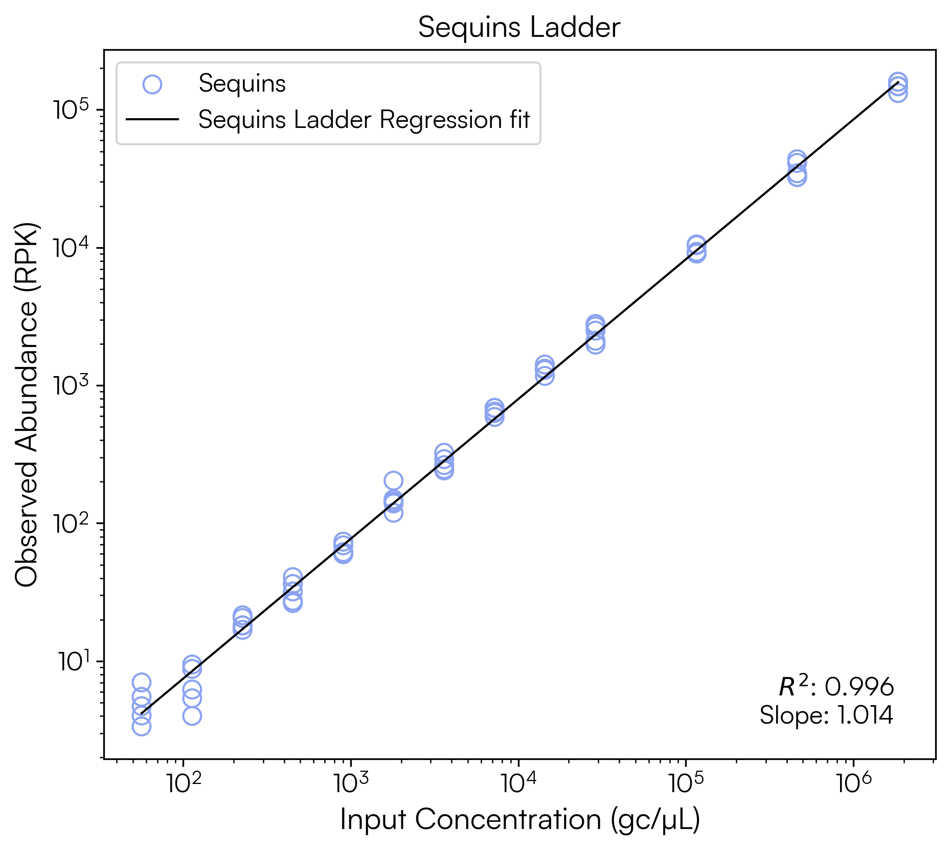
The regression yields an R² of 0.996 and a slope of 1.014, indicating good sequencing performance, with strong agreement between the expected and observed Sequins abundances and near-proportional recovery across the dynamic range.
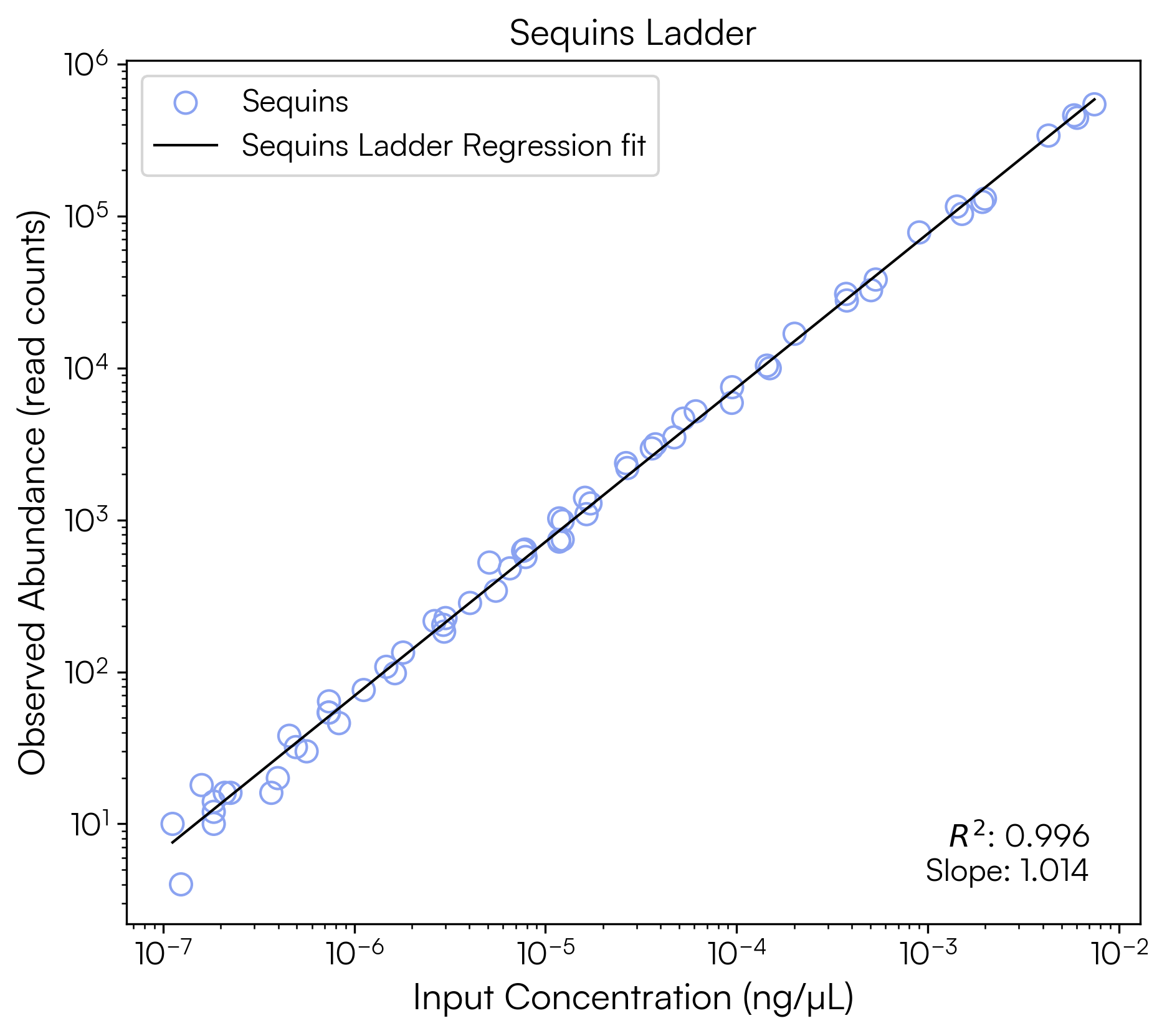
To generate a similar ladder for raw read counts against input ng/µL:
ngul_model = plot_sequins_ladder(
    sqn_df,
    'ngul',
    'read_count',
    x_label='Input Concentration (ng/µL)',
    y_label='Observed Abundance (read counts)',
    title="Sequins Ladder",
    filename=None
)
4.3 Evaluating Limit of Detection / Limit of Quantification
There are multiple methods for quantification of Limit of Detection (LOD) and Limit of Quantification (LOQ) and the appropriate approach should be selected in consideration of your experiment.
For the purpose of this tutorial we apply a simple definition of LOD as the lowest individual concentration point in the Sequins ladder at which all Sequins are detected, and define LOQ as the lowest individual concentration point in the Sequins ladder at which all Sequins are detected and at which the Coefficient of Variation (CV) is ≤ 35% for back calculated concentrations, in line with general guidelines for qPCR (Kubista et al. 2017).
In Python we can run:
loq, lod, results = limits_calculation(
    gcul_model,
    sqn_df,
    x_col='gcul',
    y_col='RPK',
    cv_threshold=35.0
)

results.to_csv('limit_calculation_summary.csv')

print(f"LoD = {lod:.3e}")
print(f"LoQ = {loq:.3e}")
Which returns both our LoD and LoQ for this sample as 56.4 copies/µL, and a summary of the results at each point in the Sequins ladder:
LoD = 5.640e+01
LoQ = 5.640e+01
| known_input_concentration | all_detected | mean_backcalc | std_backcalc | cv_percent |
|---|---|---|---|---|
| 5.64E+01 | TRUE | 6.62E+01 | 1.87E+01 | 28.26768569 |
| 1.13E+02 | TRUE | 9.05E+01 | 3.04E+01 | 33.52436372 |
| 2.26E+02 | TRUE | 2.52E+02 | 2.49E+01 | 9.885758225 |
| 4.51E+02 | TRUE | 4.27E+02 | 7.78E+01 | 18.23865095 |
| 9.02E+02 | TRUE | 8.46E+02 | 7.62E+01 | 9.008756759 |
| 1.80E+03 | TRUE | 1.94E+03 | 4.00E+02 | 20.6303501 |
| 3.61E+03 | TRUE | 3.49E+03 | 4.32E+02 | 12.38874014 |
| 7.22E+03 | TRUE | 8.16E+03 | 5.06E+02 | 6.198245616 |
| 1.44E+04 | TRUE | 1.62E+04 | 1.08E+03 | 6.638424459 |
| 2.89E+04 | TRUE | 2.98E+04 | 4.34E+03 | 14.5484886 |
| 1.16E+05 | TRUE | 1.18E+05 | 8.76E+03 | 7.452586918 |
| 4.62E+05 | TRUE | 4.40E+05 | 6.12E+04 | 13.92872057 |
| 1.85E+06 | TRUE | 1.75E+06 | 1.30E+05 | 7.428989412 |
Sequins abundance values and the Sequins log-log model calculated with this tutorial can be used for further downstream analyses, such as normalisation of microbial species abundances to Sequins and comparison of microbial species abundances between samples. Please refer to the Sequins Publications Guide for examples of applications of Sequins in analysis of metagenomics data.